Example Scripts
Morphology of of a Single Black Carbon Particle
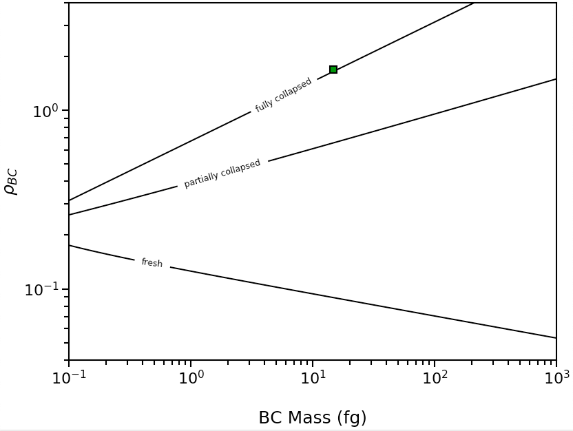
To infer the morphology of a single BC particle, use the abs2shape_SP() function. This example shows a particle with mass-equivalent diameter of 250nm, Mtot/MBC of 10, and MACBC of 12.5 m2/g measured at 532 nm, coated with non-absorbing material.
>>> import pyBCabs.retrival as pyBCabs
>>> pyBCabs.abs2shape_SP(250, 10, 12.5, 532, k_coat=0.00, ReturnPlot=False, PlotPoint=True)
{'mass': 14.726215563702151,
'rho_lower': 1.6958737655127754,
'rho': 1.6958737655127754,
'rho_upper': 1.6958737655127754}
This particle has \({\rho}\)BC > 1, and generates this morphology plot:
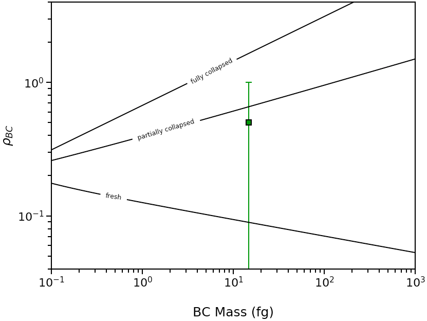
If the measured MACBC were 15 m2/g, then 0 < \({\rho}\)BC < 1, and this morphology plot will be generated:
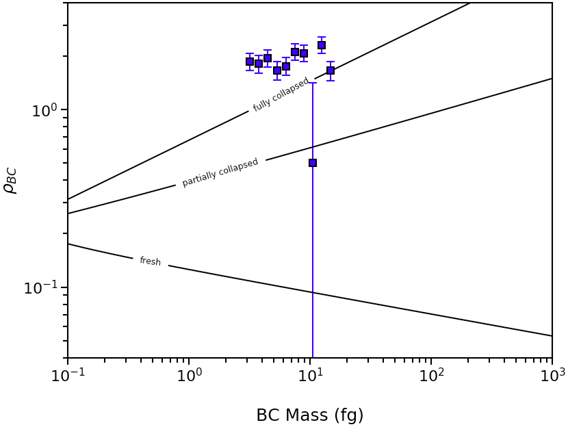
If you wish to plot multiple particle-resolved measurements, this can also be done using the abs2shape_SP() function.
wl=532 #wavelength
dp=np.logspace(np.log10(150),np.log10(250),10) #example BC mass-equivalent diameter measurements
M=10 #coating amount
p_avg=np.zeros(len(dp))
lower=np.zeros(len(dp))
upper=np.zeros(len(dp))
mass=np.zeros(len(dp))

fig, ax, result = pyBCabs.abs2shape_SP(1, M, 6.4, wl, k_coat=0.0, abs_error=1.0, ReturnPlot=True, PlotPoint=False)

for i in range(0,len(dp)):

    MAC=np.random.normal(0.8,0.1)*15
    result=pyBCabs.abs2shape_SP(dp[i], M, MAC, wl, k_coat=0.0, abs_error=1.0, ReturnPlot=False, PlotPoint=False)
    mass[i]=result['mass']
    p_avg[i]=result['rho']
    lower[i]=result['rho']-result['rho_lower']
    upper[i]=result['rho_upper']-result['rho']

errors=np.row_stack((lower,upper))
ax.errorbar(mass, p_avg, yerr=errors, markersize=7, fmt = 's', mfc='b', mec = 'k', capsize=4, ecolor = 'b', elinewidth=1.5, mew=1.5)
plt.show()
The above code will generate a plot similar to this:
Absorption of of a Single Black Carbon Particle
To calculate MACBC of a single particle, use the shape2abs_SP() function. This example shows a partially collapsed BC particle with mass-equivalent diameter of 250nm and Mtot/MBC of 10, calculated at 532 nm, with non-absorbing coating.
>>> import pyBCabs.retrival as pyBCabs
>>> pyBCabs.shape2abs_SP(250, 10, 'partial', 532, k_coat=0.00, mode='MtotMbc', r_monomer=20, asDict=True)
{'dp': 250,
'coating': 10,
'MAC': 15.270921290660958}
Morphology of Black Carbon Size Distribution
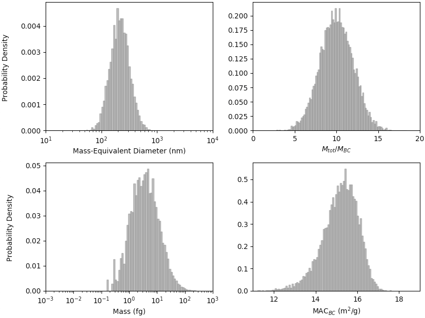
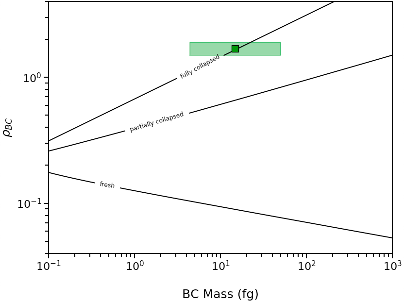
To infer the morphology of a lognormal size distribution of black carbon particles, use the abs2shape_SD() function. This example shows a distribution of black carbon with geometric mean mass-equivalent diameter of 250nm, geometric standard deviation of 1.5, Mtot/MBC of 10, and MACBC of 12.5 m2/g measured at 532 nm, with non-absorbing coating.
>>> import pyBCabs.retrival as pyBCabs
>>> pyBCabs.abs2shape_SD(250, 1.5, 10, 12.5, 532, k_coat=0.0, abs_error=1.0, ReturnPlot=True)
<Figure size 832x624 with 1 Axes>,
<matplotlib.axes._subplots.AxesSubplot object at 0x119e22e80>,
{'min_mass': 4.363323129985816,
'avg_mass': 14.726215563702134,
'max_mass': 49.70097752749473,
'rho_lower': 1.4961402652726399,
'rho': 1.6958737655127754,
'rho_upper': 1.9011038545429513}
 >>> plt.show()
The above code will generate the following plot:
Absorption of of a Black Carbon Size Distribution
To calculate MACBC of a lognormal black carbon size distribution, use the shape2abs_SD() function. This example shows a partially collapsed black carbon size distribution with geometric mean mass-equivalent diameter of 250nm, geometric standard deviation of 1.5, and Mtot/MBC of 10 (with standard deviation of 2), calculated at 532 nm, with non-absorbing coating.
>>> import pyBCabs.retrival as pyBCabs
>>> pyBCabs.shape2abs_SD(250, 1.5, 10, 2, 'partial', 532, k_coat=0.00, mode='MtotMbc', r_monomer=20, DataPoints=False, ShowPlots=True)
{'dp_avg': 271.1435259574555,
'dp_stdev': 115.42341830345885,
'coating_avg': 9.989282292286155,
'coating_stdev': 1.9791873855346263,
'MAC_avg': 15.165034433016245,
'MAC_std': 0.8543285503019649}
The following plot is also generated: